Why a 99 GB Model OOMs on 121 GB Memory: LLM Inference Internals on a Single DGX Spark

A few days ago I went down a rabbit hole that started with a deceptively simple question: if a model checkpoint is 99 GB and your target machine offers 121 GB of unified memory, why does it crash with an out of memory error the moment you run generation?

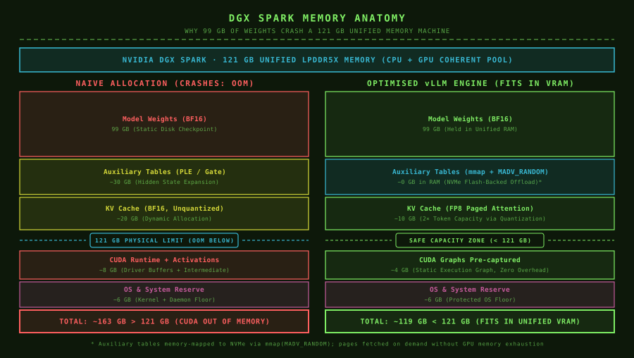
On paper, 121 GB minus 99 GB leaves 22 GB of breathing room. In practice, a naive deployment on an NVIDIA DGX Spark crashes almost immediately.

That question turned into a multi-day deep dive into the systems mechanics of modern inference engines like vLLM: key-value (KV) caching, NVFP4 and FP8 quantization, CUDA graphs, memory-mapped auxiliary table offloading, and the decisive role hardware topology plays in serving throughput.

I took notes while studying MiaAI-Lab's recipe for running Qwen 3.8 Flash Next on a single DGX Spark. Putting the pieces together helped me build an intuitive mental model for what actually happens under the hood during large language model serving.

The naive assumption that gets everyone

When you first calculate hardware requirements, it is natural to treat model weights as the only significant cost. A 99 GB checkpoint fits comfortably into 121 GB of physical memory. You load the model, call generate, and expect smooth execution.

Except it fails. You get an immediate CUDA out of memory error (NV_ERR_NO_MEMORY), and it feels baffling because the basic subtraction checked out.

The issue is that the static checkpoint size only accounts for frozen parameters sitting at rest on disk. It completely ignores what happens the millisecond real inference begins:

1. The dynamic KV cache: Every single token generated across every concurrent user stream appends new keys and values to an attention history that grows continuously.
2. Intermediate activation memory: Layer-by-layer tensors generated during attention, linear projections, and normalization layers during the forward pass.
3. CUDA runtime scratchpads: Memory reserved by CUDA driver pools, execution workspaces, and cuBLAS/CUTLASS temporary buffers.
4. The 30 GB auxiliary table surprise: Modern architectures often bundle large auxiliary embedding tables alongside the primary transformer layers, which are not reflected in standard weight summaries.
5. Operating system and driver reserves: On unified memory systems, if host memory falls below safety thresholds (such as 6 GB), kernel watchdogs terminate processes to prevent total system freezes.

Inference is not a simple "does the model fit" question. It is an active memory and bandwidth budgeting problem.

The twin phases: why prefill and decode fight each other

To understand why memory management is so critical, you have to recognize that LLM inference is not one uniform workload. It is two fundamentally different execution phases stitched together in a single loop.

Prefill is compute-bound

Prefill processes the entire input prompt in one shot. If a user submits a 32,000-token prompt, the model calculates self-attention and matrix multiplications across all 32,000 tokens simultaneously.

Because large matrix-matrix multiplications (GEMM) can saturate the GPU's arithmetic execution pipelines, prefill is heavily compute-bound. The limiter is the raw tensor core floating point throughput (FLOPs) of the chip.

Decode is memory bandwidth-bound

Once the prompt is ingested, generation shifts into autoregressive decode. The model generates exactly one token, appends it to the sequence history, and repeats the cycle.

Unlike prefill, decode runs small matrix-vector multiplications (GEMV). For every single token produced, the hardware must read the entire model weight footprint and the entire historical KV cache out of memory, only to compute math on a single token vector.

Decode is therefore strictly memory bandwidth-bound. The arithmetic units sit idle waiting for memory buses to deliver weights and cached states.

Multi-user contention

In production, an inference engine does not serve a single request in isolation. It handles multiple concurrent streams, such as 4, 8, or 16 active users.

At any given moment, a long 64,000-token prefill from one incoming request and active decode steps for seven other users are running on the same GPU. They fight for the exact same memory pool, the same memory bus, and the same attention cache.

If a long prefill takes 15 seconds of undivided GPU time, every other user's stream freezes for 15 seconds, creating terrible Time to First Token (TTFT) and high jitter.

The optimization stack

Fitting a 99 GB Qwen model onto a single 121 GB DGX Spark requires solving both the capacity bottleneck and the bandwidth wall. The solution is an interconnected stack of systems engineering optimizations.

1. The 30 GB surprise: memory-mapped PLE offloading

The most surprising discovery in this architecture was the auxiliary table footprint.

Beyond the primary transformer weights, models with deep parameter-level embeddings (such as specialized vision-language components or routing tables) can carry auxiliary structures adding 27 to 30 GB on top of the base 99 GB checkpoint. If you attempt to load both directly into unified RAM, your baseline static requirement balloons to ~128 GB, exceeding the 121 GB device limit before allocation even begins.

Compressing the table further is not strictly necessary. The real insight is recognizing that the entire table does not need to sit in memory at once.

During inference, token lookups across these auxiliary tables are sparse. Instead of holding all 30 GB in physical RAM, the engine writes the packed table to fast NVMe SSD storage and maps it into the virtual address space using the POSIX mmap system call with MADV_RANDOM.

# Conceptual memory-mapped auxiliary table loader
import mmap
import os
import torch

def load_mapped_auxiliary_table(filepath: str, shape: tuple, dtype=torch.float16):
    file_size = os.path.getsize(filepath)
    with open(filepath, "r+b") as f:
        # Map file directly to virtual memory without reading it into RAM
        mapped_buffer = mmap.mmap(f.fileno(), 0, access=mmap.ACCESS_READ)
    
    # Wrap mapped buffer directly into a PyTorch tensor
    storage = torch.UntypedStorage.from_buffer(mapped_buffer, byte_order="native")
    table_tensor = torch.empty(shape, dtype=dtype).set_(storage)
    return table_tensor

The mental model is having a vast personal library in a storage unit next door rather than cluttering your living room floor. You do not need all 10,000 books in your hands; you only fetch the specific chapter you are reading right now.

Because page faults on a cold gather can stall execution, the engine batches sparse reads using posix_fadvise(WILLNEED). Prefetching missing 4 KiB pages ahead of the token gather routine delivers a massive 13x speedup on cold row lookups during prefill.

2. FP8 KV caching: reclaiming 40 GB of headroom

After static weights, the key-value cache is the largest consumer of memory. Storing keys and values in standard 16-bit precision (BF16 or FP16) requires 2 bytes per element:

$$\text{KV Bytes per Token} = 2 \times (\text{layers}) \times (\text{KV heads}) \times (\text{head dimension}) \times (\text{bytes per element})$$

For deep models with large contexts, a few concurrent streams will easily consume tens of gigabytes of KV memory.

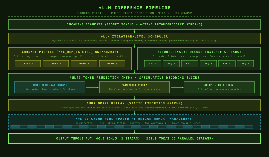
By switching the KV cache storage data type to FP8 (specifically 1 byte per element with per-tensor or per-channel scaling), memory consumption is cut cleanly in half. On the DGX Spark, configuring KV_CACHE_DTYPE=fp8 allows an allocated 16.5 GB KV pool to hold approximately 992,584 tokens. That represents almost 1,000,000 tokens of cache headroom, enough to sustain multiple long-context requests concurrently without running out of memory.

3. Chunked prefill: ending the starvation of decode streams

When a user submits a 64,000-token prompt, running it in a single compute block monopolizes the GPU for seconds. Meanwhile, all existing generation streams stall.

Chunked prefill solves this by dividing massive prompt sequences into digestible chunks, such as 2,048 or 8,192 tokens per step (MAX_NUM_BATCHED_TOKENS=2048). The vLLM scheduler schedules one chunk of prefill, then executes a round of decode steps for active users, then schedules the next prefill chunk.

This interleaving smooths out latency spikes. While halving the chunk width introduces slight kernel scheduling overhead during prefill, it drops generation jitter dramatically, maintaining steady interactive token output across concurrent streams.

4. Speculative decoding and Multi-Token Prediction (MTP)

Since autoregressive decoding is memory bandwidth-bound, calculating tokens one by one leaves the tensor cores mostly idle. Speculative decoding addresses this imbalance by pairing the primary model with a lightweight draft head or draft model.

In an MTP setup with a speculation depth of $K=3$:

1. The small draft head rapidly guesses the next 3 tokens in sequence. Because the draft head has fewer parameters, it evaluates much faster.
2. The full target model ingests all 3 candidate tokens simultaneously in a single forward pass.
3. The target model computes cross-entropy verification across all positions in parallel.
4. Accepted candidate tokens (typically 2 to 3 out of 3 on predictable text) are committed to the output stream immediately.

Instead of paying the full model memory-read penalty 3 separate times, you pay it once and receive up to 3 tokens.

Step 1: Draft model generates:   [ "The" ] -> [ "capital" ] -> [ "of" ]
Step 2: Target model verifies:   [ OK ]       [ OK ]            [ OK ]
Result: 3 tokens produced in the time of 1 full forward pass!

To optimize decode further, the engine implements a reduced draft vocabulary (MTP_DRAFT_VOCAB). In standard setups, the draft model evaluates logits across the full 152,000-token vocabulary table, requiring a 1.18 GB read of lm_head weights on every draft step. By restricting the draft head's vocabulary to a curated subset of 47,000 or 65,000 frequent IDs (covering 99.5% of real prose and code), the engine eliminates 2.61 GB of memory bandwidth per step.

That bandwidth reduction converts directly into speed, boosting decode rates from 36.9 tokens/sec to 46.3 tokens/sec on a single stream, and reaching 162.9 tokens/sec aggregate throughput across 8 concurrent streams.

5. CUDA graphs: removing host CPU dispatch overhead

Launching a GPU kernel requires the host CPU to submit commands across the driver stack. In autoregressive decoding, where small kernels execute thousands of times in rapid succession, CPU driver latency frequently exceeds actual GPU compute time.

CUDA graphs capture a complete sequence of kernel launches, memory bindings, and dependency barriers once during initialization. During active generation, the engine replays the entire execution graph with a single hardware launch call. This eliminates the CPU dispatch overhead, ensuring the GPU's memory controllers remain continuously saturated.

6. BF16 recurrent state caching

For hybrid architectures incorporating linear attention or recurrent SSM layers (such as Mamba-style state blocks), state variables must be maintained across steps.

While attention KV caches benefit from 8-bit quantization, keeping recurrent state representations in bfloat16 (MAMBA_SSM_CACHE_DTYPE=bfloat16) preserves numerical stability without consuming excessive memory. Benchmarks show this configuration delivers an 8.5% throughput gain at 8 concurrent streams compared to lower-precision recurrent accumulation.

Hardware topology: why memory capacity is only half the story

When developers evaluate hardware for LLM serving, they usually look at a single metric: total memory in gigabytes. But physical memory layout and interconnect bandwidth dictate what parallel strategies are practical.

Unified memory architectures (DGX Spark)

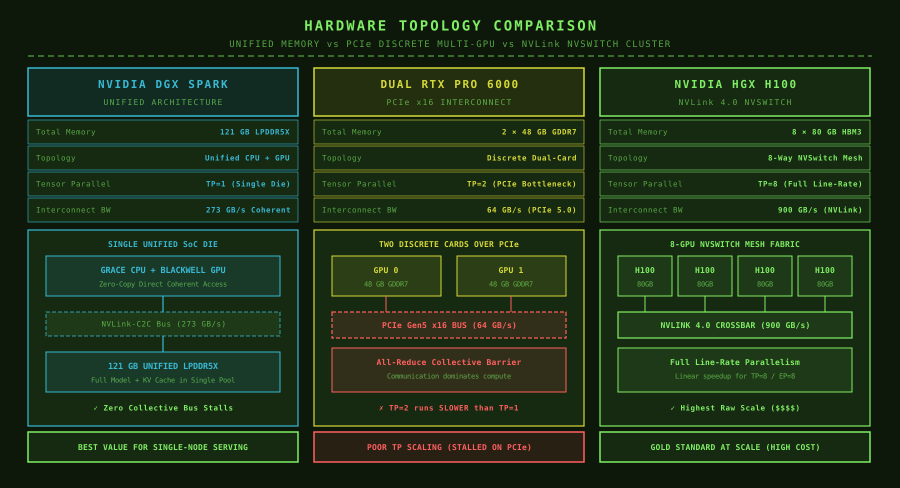
The NVIDIA DGX Spark features a unified memory architecture where CPU cores and GPU tensor cores share a coherent 121 GB LPDDR5X memory space.

This topology has two distinct properties:

• Advantage: Zero-copy sharing between host and accelerator. Memory-mapped NVMe offloading works efficiently because the operating system's page cache and the GPU's virtual memory space operate across the same physical RAM.
• Constraint: There is only one hardware device, meaning Tensor Parallelism ($TP=1$) is fixed. Furthermore, you must maintain a strict HOST_RESERVE_GIB (such as 24 to 26 GB) so that background Linux processes, TCP networking buffers, and container runtimes never starve, which would trigger kernel panics.

Discrete multi-GPU over PCIe

Consider a dual-GPU workstation with two 48 GB RTX Pro 6000 cards connected via a standard PCIe Gen4 x16 bus. While total memory appears to be 96 GB, the GPUs are separated by a relatively narrow 64 GB/s channel.

If you attempt to run Tensor Parallelism ($TP=2$) across these cards, every attention and MLP layer must exchange activations via all-reduce operations across the PCIe slot. The PCIe bandwidth is so much slower than internal VRAM bandwidth (>1,000 GB/s) that communication latency completely erodes compute speed. In many cases, splitting a model across PCIe cards runs slower than serving a quantized checkpoint on a single node.

NVLink clusters (H100 / HGX)

Enterprise AI nodes use dedicated NVLink interconnects and NVSwitch fabrics, delivering 900 GB/s of bidirectional bandwidth between GPUs.

Only at these interconnect speeds does fine-grained Tensor Parallelism ($TP=8$) or Expert Parallelism ($EP=8$ across Mixture of Experts layers) scale efficiently. The inter-GPU communication is fast enough to keep up with arithmetic execution pipelines.

What this means for AI systems engineering

Going into this investigation, I assumed that fitting a 99 GB model was a simple quantization task: convert weights from 16-bit to 4-bit, launch the container, and finish.

Instead, I found that high-throughput LLM serving is an end-to-end systems balancing act:

• Weights are just the floor: Static parameters are only the starting point. Unmanaged KV caches and hidden auxiliary tables will easily overwhelm available capacity.
• Memory mapping turns storage into virtual headroom: Using mmap with asynchronous readahead allows tens of gigabytes of sparse auxiliary parameters to live on fast NVMe drives rather than consuming precious physical RAM.
• Bandwidth dictates decode speed: Because autoregressive decoding is memory-bound, reducing KV precision to FP8 and shrinking draft vocabulary tables produces immediate, measurable token rate improvements.
• Hardware interconnects determine architecture: Compute power cannot compensate for slow communication channels. Squeezing maximum throughput out of a single unified-memory node frequently outperforms poorly interconnected multi-GPU clusters.

Managing inference is fundamentally a memory and bandwidth budgeting problem. Once you understand where each byte goes and how the phases interact, running massive models on constrained hardware shifts from an exercise in frustration into an elegant systems problem.

Keep reading

• MiaAI-Lab Qwen3.8-Flash-Next Single DGX Spark Recipe (GitHub repository and benchmark sweep scripts)
• What is a KV Cache? explains key-value state retention and memory overhead
• What is Paged Attention? covers non-contiguous memory management in vLLM
• What is Speculative Decoding? dives into draft model verification mechanics
• What is Continuous Batching? breaks down dynamic iteration-level request scheduling
• GPU Architecture Explained covers streaming multiprocessors, memory tiers, and warp scheduling